The theory behind computational topology, along with intuitive examples
Overview
To round off day 1, we combine what you learned in the first two sessions to cover the basics of topological data analysis (TDA). While learning the requisite theory, we present relevant examples in R in order to gain hands-on experience with TDA.
This session is presented jointly by Brittany and Ben. Brittany will cover most of the theory, and Ben will lead R programming sections.
Objectives: After this session, we hope you will be able to:
Recognize topological shape in data
Define a filtration, and give at least two examples of different filtrations
Explain persistence barcodes/diagrams at a high level
Create the Vietoris-Rips and other complexes in R
Compute a persistence diagram in R
1.Getting Started
We begin this session by introducing simplicial complexes in R.
Create a new R script for this session in your project, and name it session-3. This afternoon we’re getting our feet wet with topological data analysis, so we’ll need to install and import the R TDA package.
install.packages("TDA")
library(TDA)
In the R TDA package, simplicial complexes are typically represented as lists. Remember they are quite simple to create:
myFirstList <- list(1, TRUE, "There's a string in my list too!")
Knowing this, we can create a simplicial complex using only the list() and c() functions to create a list object and combine function, which we saw earlier. Typically, we label each vertex in a simplicial complex with an integer, and build the complex accordingly. Here’s how to do it for two vertices joined by an edge.
simpleK <- list(1, 2, c(1,2))
Try it yourself! See if you can create the simplicial complex in the example above, combinatorially defined by the set $A$.
Now, you might be wondering, “how could I go from typical data, like a set of points, to a simplicial complex?”
Once we have a simplicial complex representing our data, we can compute homology and other topological invaraints. Thus, finding a simplicial complex from data gives us the tools necessary to find topology in data. It turns out that there are tons of ways to study topology in point cloud data.
As a first example, we consider point cloud data. That is, a point cloud, $S \subset \mathbb{R}^n$, is a finite set of points in (usually Euclidean) space. Such data sets arise in many ways. Mathematically, maybe there is an underlying, unaccessible shape that we can sample from (such as the torus):
Note that manifolds (like the torus) can represent various things. For example, the torus parameterizes the configuration space of a two-arm linkage (with one fixed point).
Other examples of point cloud data can come from locations, such as locations of speed traps or wildfires.
Once we have a point cloud, we need to organize it. You may be familiar with contact graphs where the represent a geometric object such as a circle, curve, or polygon, and an edge between two vertices exists if the corresponding two objects intersect. The Vietoris-Rips (VR) complex, which we investigate next, is a generalization of contact graphs.
Let $S$ be finite set of points in $\mathbb{R}^n$. Let $r\geq 0$. The Vietoris-Rips (VR) complex of $S$ and $r$ is the abstract simplicial complex, denoted $\text{VR}(S, r)$, consisting of all subsets of diameter at most $r$:
$ \text{VR}(S, r):=\{\sigma\subset S \mid \text{ diam}(\sigma)\leq r \}, $
where the diameter of a set of points is the maximum distance between any two points in the set.
Geometrically, we constuct the Vietoris-Rips (VR)-complex by considering balls of radius $\frac{r}{2}$, centered at each point in $S$. Whenever we have a set of $n$ balls that pairwise intersect, we add an $n-1$ dimensional simplex. Consider the following sets and their corresponding simplex:
Checking all subsets of $S$, we can find our a simplicial complex:
More Info
The VR-complex is an approximation of the Čech complex.
The Čech complex is an abstract simplicial complex that is homotopy
equivalent to a union of balls.  It is created by adding a vertex for each ball,
an edge between vertices correspoding to intersecting balls (so far, we're in
the same setting as the Rips filtration), and adding an $n$-simplex for each
$(n+1)$-way intersection of balls. To see where they differ, consider the
two-complex above that is created when three balls pairwise intersect in the
VR-complex.  If there is not a three-way intersection, the triangle is not
added to the Čech complex.


Čech complex.
2. Filtrations
The Vietoris-Rips Filtration
In the VR-complex, $r$ is a parameter. If we vary $r$, we get different VR-complexes. So, which one do we pick? In many data analysis situations, the value of $r$ that best describes the data is unknown or does not exist, so why not look at all of them!? Observe if we increase $r$ continuously, the complex only changes a finite number of radii, say at $r_0 < r_1 < \ldots < r_n$. Then, we get a family of nested VR-complexes that we call the Vietoris-Rips filtration (or simply the Rips filtration).
More generall, a filtration of a simplicial complex, $K$, is a nested sequence of subcomplexes starting at the empty set $\emptyset$ and ending with the entire complex $K$.
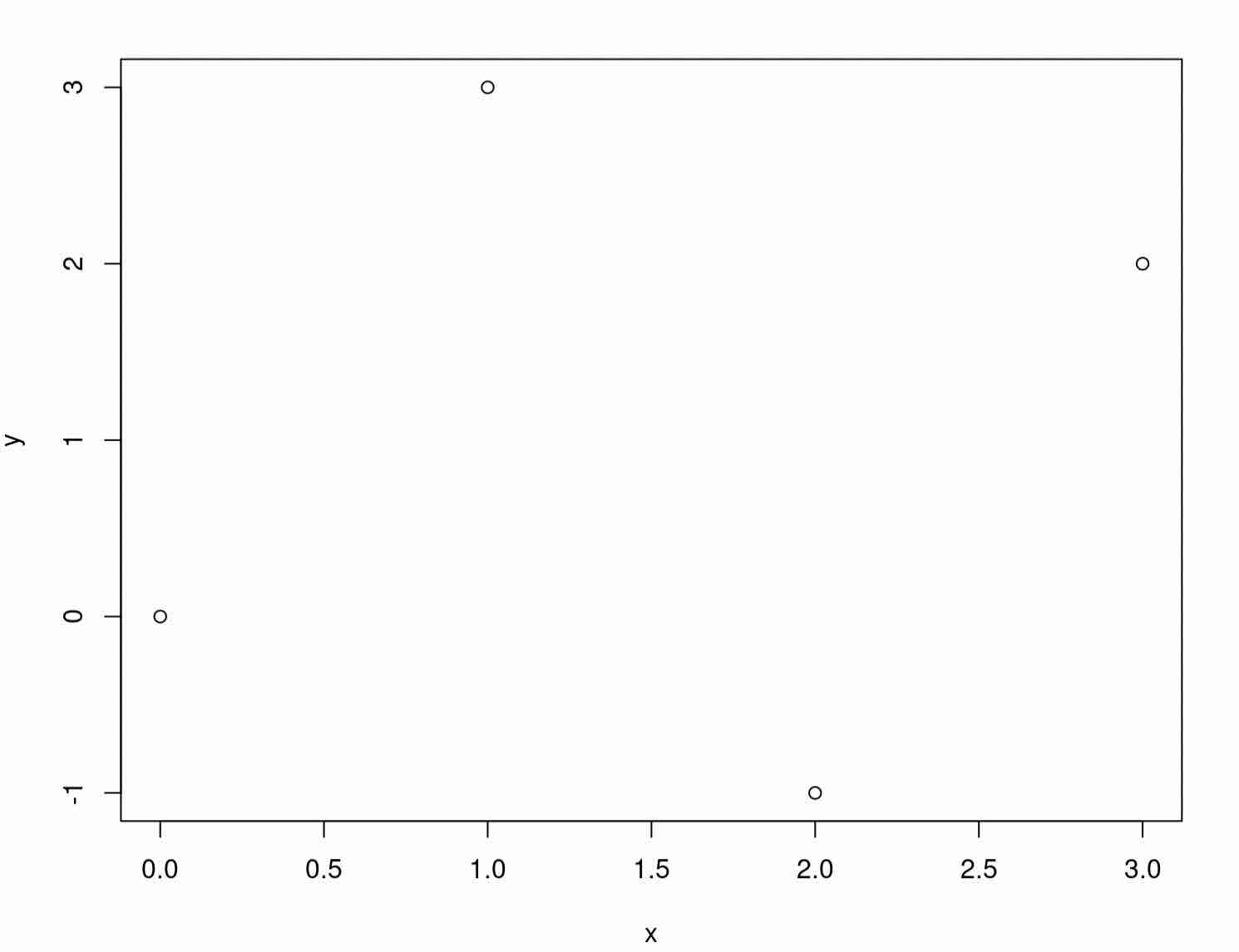
Let’s work through an example. Let $S:={(0,0),(1,3),(2,-1),(3,2)}\subset \mathbb{R}^2$. For a visualization, this is easy to plot in R:
x <- c(0,1,2,3)
y <- c(0,3,-1,2)
plot(x=x, y=y)
Expected Output
We want to compute a Rips filtration on $S$ for all $r\geq 0$.
Observe:
When $r<\sqrt{5}$, none of the balls of radius $\frac{r}{2}$ intersect and so $\text{VR}(S,r$) is four points.
When $r=\sqrt{5}$, the balls of radius $\frac{\sqrt{5}}{2}$ centered at $(0,0)$ and $(2,-1)$ intersect which means we add a 1-simplex between $(0,0)$ and $(2,-1)$. Similarly, we add a 1-simplex between $(1,3)$ and $(3,2)$.
When $r\in (\sqrt{5},\sqrt{10})$, no additional balls of radius $\frac{r}{2}$ intersect which means $\text{VR}(S, r)=\text{VR}(S, \sqrt{5}$).
When $r=\sqrt{10}$, we add a two more 1-simplices between $(0,0), (1,3)$, and $(2,-1), (3,2)$.
When $r \in (\sqrt{10},\sqrt{13})$, $\text{VR}(S,r)=\text{VR}(S, \sqrt{10}).$
When $r=\sqrt{13}$, we add two 2-simplices between $(0,0),(1,3),(2,-1)$ and $(1,3),(2,-1),(3,2)$.
When $r \in (\sqrt{13},\sqrt{17})$, $\text{VR}(S,r)=\text{VR}(S, \sqrt{13}).$
When $r=\sqrt{17}$, we add a 3-simplex.
When $r>\sqrt{17}$, $\text{VR}(S,r)=\text{VR}(S, \sqrt{17}).$
Hopefully the Vietoris-Rips filtration, and the idea behind filtrations more generally, is clearer with an example in mind.
If not, we also made a movie:
A Rips Filtration in R
In R, we can use the ripsFiltration function in the TDA package to conduct filtrations. Let’s try it out for $r<\sqrt{5}$, using the same four example points from above. If $r<\sqrt{5}$, above, we noted that the complex is simply four points.
# create our cloud of four points
x <- c(0,1,2,3)
y <- c(0,3,-1,2)
X <- cbind(x,y)

# set largest allowed radius of balls < sqrt(5)
mymaxscale <- 2

# set other necessary parameters (more on those to come)
mymaxdimension <- 4
mydist <- "euclidean"
mylibrary <- "Dionysus"

# conduct Rips filtration
FltRips <- ripsFiltration(X = X, maxdimension = mymaxdimension,
                          maxscale = mymaxscale, dist = mydist, library = mylibrary,
                          printProgress = TRUE)
Try on your own to view the resulting Rips complex, and see if it confirms what we thought the final complex should be above. (HINT: to view the Rips complex, you will need to use the $ syntax for attributes of the filtration)
Now that we have a good sense of Vietoris-Rips complexes, and the filtration that results treating $r>0$ as a free variable, we now will discuss useful data structures to store and interpret filtrations.
Keep this example in your workspace, as we will come back to it shortly.
Images and Lower-Star Filtrations
The Rips filtration is great for creating connections within a point cloud. However, sometimes, we already know what these connections are. And, many times there is a function defined over the topological space that is of interest. A simple example to start is an image. The underlying topological space is a square or a rectangle (pretty boring topologically). Images decompose this square domain into smaller squares called pixels and assign a color to each pixel. We’ll restrict ourselves to monochromatic images, so we can think of the color as a number between $0$ and $1$.
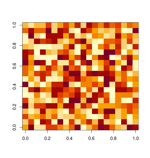
In R, let’s create and plot a random image:
n=20
vals <- array(runif(n*n),c(n,n))
image(vals)
Expected Output
To construct a complex that represents an image, we create a vertex for each pixel, add an edge between vertices if their pixels are adjacent. From here, we can add squares to get a cubical complex, and draw diagonals in the squares if we want a simplicial complex. Here’s a small example:
What you might notice is that we started with a discrete set of function vales, one for each pixel. The vertices of our complex can inherit that value. But, what value do we assign to the edges and two-cells? Discuss some ideas with your neighbors.
See the Answer
There are various ways that we can do this, actually.  The one that we will use
today assigns to each cell the maximum value assigned to any of the vertices
defining the cell.  By doing so, every lower-level set (collection of cells
below a given value) is a complex.  By considering the increasing sequence of
such subcomplexes, we arrive at the lower-star filtration.
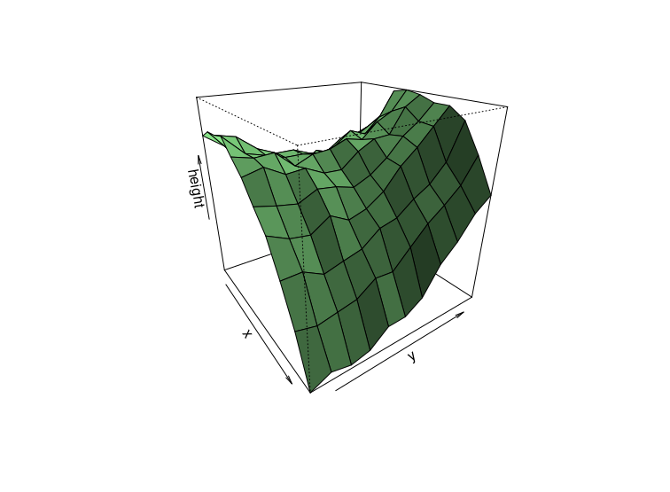
For images, the function is actually a surface created by raising each vertex up to the height equal to it’s function value. Then, edges and two-cells are interpolated. The lower-star filtration is exactly the one that arises by raising our “height” parameter and considering subcomplex of the surface that appears entirely at or below the current height parameter. Here’s a quick example to demonstrate:
newfcn <- function(x, y){jitter(-2*x^2+y^2+x+3*y-6*x+x*y,30)}
x <- seq(-5,5)
y <- seq(-5,5)
persp(x,y,outer(x,y,newfcn),zlab="height",theta=55,phi=25,col="palegreen1",shade=0.5)
Expected Output
We can contruct the lower-star filtration from the values in our image as follows:
The output is a complex of 11 simplices, along with a function value assigned to each simplex. Can you find what those simplices and function values are? (Hint: the output of gridFiltration has attributes $cmplx and $values that stores the simplicial complex and function values for each simplex, respectively).
See the Answer
To see the list of simplices in the complex:

> myfilt$cmplx
[[1]]
[1] 4

[[2]]
[1] 3

[[3]]
[1] 4 3

[[4]]
[1] 2

[[5]]
[1] 4 2

[[6]]
[1] 1

[[7]]
[1] 2 1

[[8]]
[1] 3 1

[[9]]
[1] 4 1

[[10]]
[1] 4 1 2

[[11]]
[1] 4 3 1


And the function values:

> myfilt$values
 [1] 0.1952117 0.4001437 0.4001437 0.5358404 0.5358404 0.6333039
 [7] 0.6333039 0.6333039 0.6333039 0.6333039 0.6333039
Again, keep this example in your workspace, as we will come back to it shortly.
3. Introduction to Persistent Homology: Barcodes and Diagrams
Let’s step back for a moment and think of a painting. Museums and art experts vary on their advice for the best distance to stand from a painting or print:
Lightscape Creations says to first “measure the diagonal of the [artwork] from bottom left corder to the top right corner”. Then, the viewer should be at a distance equal to 1.5 to 2 times the diagonal.
John Paul Caponigro also uses the diagonal in his calculation, but says that the viewer should be three times the diagonal away.
J Ken Spencer advocates for the 20-6-1 rule; that is, there are three distances: 20 feet, 6 feet, and 1 foot away fom the artwork.
Let’s give this a try. Setup in groups of 3. Hold up a picture. Identify three features of this photo. Mark the ground with a strip of masking tape to represent the interval of distances you can see the features clearly. For example, you can use Starry Night by Van Gogh:
The strips of masking tape create a barcode. The endpoints of the strip are placed at the minimum and maximum distances that you can view that feature. Is it possible
See Example Answer
Example barcode for select features in Starry Night. Note that in order to
see the constellation Aries, you need to stand far away from the painting that
you can no longer see individual brush strokes. So, one viewing distance is not
enough.  And, in data, often, one scale is not enough.
Now is a good time for a quick break (if we haven’t taken one recently).
Diagram for a Rips Filtration
Back to our Rips filtration, we can see that for certain $r$, homology features are either being created (e.g., loop forming) or going away (e.g., loop being filled in). Let’s look more closely at the example from before.
For example, when $r=0$, we have four connected components (just the vertices). When $r=\sqrt{5}$, we only have two connected components. When $r=\sqrt{10}$, we have only one connected component, but also note that a nontrivial one-cycle appears. It would be nice if there were some clean way to keep track of this information …
Fortunately, persistence barcodes and persistence diagrams can do just that! Persistence tracks the parameters (time, distance, height) at which a homology feature is “born” $b$ as well as when the same feature “dies” $d$. Barcodes encode this as an interval $(b,d) \subset \mathbb{R}$. Persistence diagrams encode this as a point $(b,d) \in \mathbb{R}^2$.
More Info
There is more to it than we say here. A feature of the underlying topological
space ($K$) is called an essential class and never dies.  Thus, the death
parameter can be infinite.  For this reason, we often use the extended real
plane $\overline{\mathbb{R}}^2$,
where $\overline{\mathbb{R}}=\mathbb{R} \cup \{ \infty \}$.
Even more generally, the parameter space can be an arbitrary
poset.  But, that is more than we need in T4DS.
The R TDA package has a function ripsDiag that creates diagrams corresponding to the Rips filtration. Let’s view the barcode resulting from our example filtration:
Here, 1d homology (corresponding to the connected components) is represented in black, and 2d homology (corresponding to the one-cycles) is in red. We can track the birth and death of the connected components as well as the one-cycle, by seeing the parameters at which segments begin and end in the barcode.
So, being able to plot it is great, but what if we want to work with the function values (e.g., in order to compare two diagrams)? We do have direct access to the coordinates of all points.
Finally, if you want to see the persistence diagram instead of the barcode, use:
plot(persistDiag[["diagram"]])
Expected Output
The barcode and the diagram are visualizations of the same information: the persistence of homoology generators as a parameter changes. Some researchers prefer one visualization over an another, but they’re ultimately the same object. How you might be inclined to work with them might differ based on your choice.
Diagram for a Lower-Star Filtration
Recall the image vals that we created above. There is a function in the R package TDA that computes the persistence diagram:
Change $n$ and recompute the diagram. What pattern do you see?
See the Answer
Overall, the zero-dimensional persistence points (black dots) are to the left
and below the one-dimensional ones (red triangles).  This makes sense, as in
order for loops to form, there have to be connected components first. The
pattern that arises here is something that has been studied, and can be used for
hypothesis testing (is my image just pure random noise, or is there a feature
hidden in there?)
Other Filtrations and Diagrams
The general framework of persistence is this: there is an underlying topological space, $K$, and a “nice” function $f : K \to \mathbb{R}$. The co-domain is our parameter space and can represent various things: height (in a particular direction), distance (away from a point or set), time, etc. As the parameter $t$ increases, we consider all sublevel sets: $f^{-1}(-\infty,t]$. These are subcomplexes of $K$ (or else $f$ was not “nice”). Here’s another example that we call “the (upside down) V example”:
In our example, we have a simplicial complex in $\mathbb{R}^2$ and the function $f$ takes a simplex $\sigma$ to the maximum height of any vertex in the simplex:
$ f(\sigma) = \max_{\text{vertex} v \preceq \sigma} f(v).$
Note that the height of a point (or vertex) $p \in \mathbb{R}^n$ in direction $d \in \mathbb{S}^{n-1}$ is simply the dot product $v \cdot d$. Examples to consider are polygons (representing county boundaries, for example) and 3d scanned object.
Create a complex in R to match the V-example above. (Hint: remember from earlier that a complex is a list of simplices, and a simplex is a “combination” of vertices).
See the Answer
# create vertices
a <- 1; b=2; c=3
# edges
ac <- c(1,3); cb=c(2,3)
# a complex is a list of simplices
vcplx <- list(a,b,c,ac,cb)
Next, let’s use cbind to create a data structure to store the coordiantes (note: you can make up coordinates).
See the Answer
x <-c(0,2,1)
y <- c(0,0,1)
vcoords <- cbind(x,y)
And, the final piece left is to compute the function values for the vertices! Like above, we can use the z-coordinate of the highest vertex. For now, we can do this by hand and create a numeric array. (Challenge: compute this from vcoords!)
See the Answer
vvals <- c(0,0,1)
Once we have these elements, we can use the funFiltration to create our filtration and compute the diagram as follows:
Thanks for your attention to end today’s workshop materials! To summarize our accomplishments this afternoon:
We learned about simplicial complexes, and worked with them in R
We learned about Vietoris-Rips complexes, and used them in R
We learned about filtrations
We learned about persistence diagrams and barcodes, and implemented them in R
We learned about the height filtration
Credits
This material was based on other tutorials developed by Robin Belton, Ben Holmgren (name familiar?), and Jordan Schupbach. We thank them for giving us a head start on this material!
The illustration of representing an image with a cubical or simplicial complex is from an upcoming paper by Brittany and her colleagues, Jessi Cisewski-Kehe and Dhanush Giriyan.