A Brief Introduction to Topology

Overview

In this session, we provide a light and fast introduction to the subject of topology, a field of mathematics that stems from pure mathematics, but has applications in data analysis that makes it an interesting subject to applied mathematicians, statisticians, computer scientists, data scientists, and other data scientists alike.

This session is presented by Brittany.

Objectives: After this session, we hope you will be able to:

• Define “shape”
• Describe topological and geometric properties of a space/shape
• Explain how to represent data as a complex

1. Getting Started

We are glad that you are here with us for this workshop! The first activity is hands-on, literally.

We start by standing in a circle. Then, hold hands with two differnt people (both cannot be next to you). Can we unknot ourselves?

Knot theory is fun! If we can unknot ourselves and we have formed one connected component, then we have formed the unknot, or the most basic/fundamental of all knots. If we created two cycles (each an unknot or not), then we have formed a link.

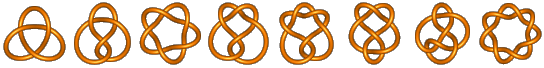
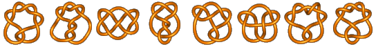
Other knots that are interesting (and not equivelent to the unknot) are the trefoil knot and the figure 8 knot. These are the first two knots of the “sixteen simplest knots”:

Variants to try (in smaller groups):

1. If you start facing each other and hold your neighbor’s hands, can you turn your circle “inside-out” and have your backs facing inward?
2. Can you form the trefoil knot?
3. What about the figure 8 knot?

2. What is Shape (in Data Science)?

What comes to mind with the following question: what is shape? Write three words that come to mind in this Slido poll, then discuss the results and your thoughts with your neighbors.

From Meriam Webster:

 
The visible makeup characteristic of a particular item or kind of items
 
Spatial form or contour
 
A standard or universally recognized spatial form



From Brittany: shape is a way of putting meaning or interpretability to a set. 

Often, when we think of shapes, we think of their geometry: length, witdth, angles, curvature, area, etc. In this workshop, we explore the topology of shape/data as well. Topology studies the connectivity between and among data.

3. Koenigsberg

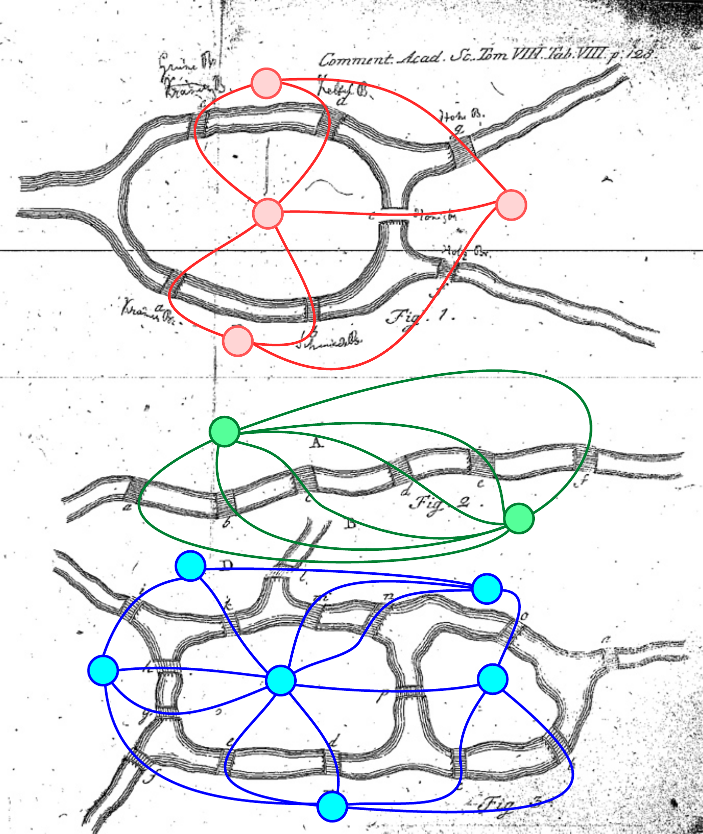
The bridges of Koenigsberg was an old problem: is it possible to walk on a path that crosses each of the seven bridges of Koenigsberg exactly once? Of course, one is not allowed to fly or swim in order to accompish this task. For the three cities shown below, discuss with your neighbors if such a path is possible. (Note: the top city is Koenigsberg).

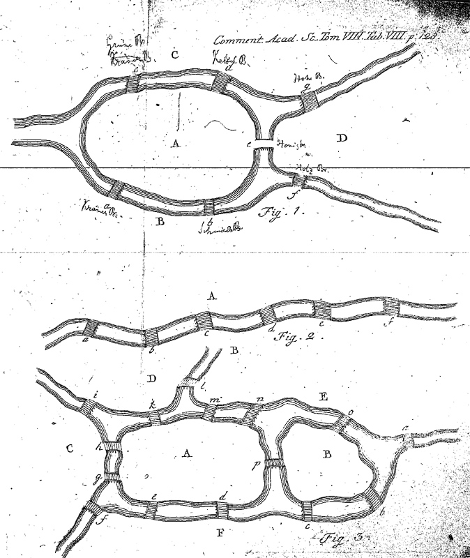
How can we solve such a question? We turn it into a topological question, of course! We do this by turning it into a graph problem. Create a graph by creating a node for each land mass or island, and creating an edge for each bridge. (This may be a multi-graph). Now, we have a graph theory problem: does there exist a path through the graph that visits every edge exactly once? Such a path is called an Eulerian path.

A Eulerian path through a graph is possible iff there exists exactly two or zero vertices of odd degree.

For each of the graphs above, can you find the corresponding graphs?

4. Are Two Shapes the Same or Different?

This is a question that we will come back to tomorrow.

First, we need to understand what a topological space is.

A topological space $(X,T)$ is a set $X$ (e.g., the real line) with a set of sets $T \subseteq 2^X$ (elements of $T$ are called open sets) that follows the following two rules:

1. The intersection of a finite number of open sets is open.
2. Any (potentially infinite) union of open sets is open.

An example is the real line, with open sets as we know them (in fact, this is called the standard topology on the reals). From now on, when we say “shape”, we mean a topological space. Often the shapes we talk about come from data.

Representing Shapes

Simplicial Complexes

Of course we are all familiar with triangles, and to understand computational topology, we must first conceptualize triangles of differing dimensions. That is, triangles of increasing dimension ranging from $0$ to $n$. (Where the -1th dimensional triangle being a null value).

Intuitively, we call an $n$-dimensional triangle an n-simplex.

More rigorously, a geometric n-simplex is the smallest convex set of $n+1$ affinely independent points. An abstract $n$-simplex is a set of $n+1$ elements (here, the elements represent the points). An $n$-simplex has $n+1$ faces of dimension $n-1$ (namely, one for leaving out each point). For example, a two-simplex has three one-dimensional faces (edges).

We say that the set of points $\{ v_0, v_1, \ldots, v_n\}$ is affinely
independent
iff the vectors $v_1-v_0,...,v_{n}-v_0$ are linearly independent.

We can collect simplices together to form a simplicial complex.

A simplicial complex $K$ is a finite collection of simplices, such that:

1. If $\sigma \in K$ and $\tau \subset \sigma$, then $\tau \in K$.
2. If $\sigma, \sigma’\in K$, then $\sigma \cap \sigma’$ is either empty or a face of both $\sigma, \sigma’$.

We can use a simplicial complex to represent shapes (and data). Then, we can interpret topological features in a computational setting.

Cubical Complexes

An $n$-cube is a copy of $I^n$, where $I$ is the unit interval $[0,1]$. A cubical complex is a topological space created by glueing cubes together along sub-cubes. A common cubical complex forms a regular grid:

A cubical complex can always be transformed into a simplicial one (namely, by adding “diagonals” to each cube). Nonetheless, quite a bit of data comes in cubical form (e.g., digital photos). So, they are also nice structures to work with.

Maps and Homeomorphisms

If we have an understanding of open sets, we can define a continuous map as:

$ f : A \to B$ is continuous iff for all open sets $U$ in $B$, $f^{-1}(U)$ is open in $A$.

The strongest form of shape equivalence is that of a homeomorphism:

Two shapes, A and B, are homeomorphic iff there exists a bi-continuous bijective map $H:A \to B$.

What this means is the perspective of $a \in A$ “looks like” the perspective of $b \in B$. In other words, the two shapes are “the same” if all you care about are the neighborhoods.

Topological Invariants

Can we explore every map $A \to B$? Nope! Instead, we study topological invariants.

A topologocial invariant $I$ is a function that takes in as input a topological space and returns a property of that space. If two spaces $A$ and $B$ are homeomorphic, then $I(A)=I(B)$. But, the reverse need to not be true.

After we introduce different invariants, see More Info for an example of two shapes that are indistinguishable up to that invariant.

Homotopy

The first invariant we consider is that of a homotopy. We’ll give the formal definition, but don’t worry too much about it if you haven’t seen it before.

Two continuous functions $\gamma_0,\gamma_1 : A \to B$ are homotopic iff there exists a continuous function $H \colon A \times I \to B$ such that $H(a,0)=f(a)$ and $H(a,1)=g(a)$ for all $a \in A$. To denote $\gamma_0$ and $\gamma_1$ are homotopyic, we write $\gamma_0 \simeq \gamma_1$.

We think of the unit interval $I$ as time and so $\gamma_0$ is “morphing” into $\gamma_1$. A common example is a homotopy between two curves in the plane. Here, $A=I$ and $B=\mathbb{R}^2$:

A nice visualization of a homotopy between two curves can be obtained by viewing $H(\cdot,t)$ as time changes with $t$, as shown in this YouTube vide. The isotopy we saw above of the donut and the coffee mug is a homotopy of two functions from the torus to $\mathbb{R}^3$. But, this is all about functions. We typically care about spaces/shapes.

We say that two topological spaces $A$ and $B$ are homotopy equivalent iff there exists continuous functions $f : A \to B$ and $g : B \to A$ such that $f\circ g \simeq \mathbb{1}$ and $g \circ f \simeq \mathbb{1}$.

We won’t dig into details here, but this roughly means that you can map $A$ to $B$ and back to $A$ in a nice way. If $f,g$ are bijections with $f=g^{-1}$ this is particularly nice (but not always possible).

A circle and an annulus are indistinguishable by homotopy equivalence alone.  
So are a [punctured torus and the wedge of two circles](https://www.youtube.com/watch?v=j2HxBUaoaPU).
In
fact, if we have two spaces $A$ and $B$ such that $B$ is a deformation retract
(think: continuously morphing by contracting) 
of $A$, then $A$ and $B$ are indistinguishable up to homotopy type.

The problem with classifying shapes up to homotopy is that they are #P-hard to compute. So, we turn to topological invariants that are easier to compute.

Euler Characeteristic

The Euler characteristic of a shape is found by first representing the shape as a cellular structure (e.g., simplicial complex or cubical complex). Then, the Euler characteristic is the alternating sum of the number of i-cells: $\chi(K) = \sum_{i=0}^{\infty} (-1)^i |K_i|$.

What is the Euler characteristic of the sphere?

    The Euler characteristic of the sphere is 2.  One topological model of the
    sphere is that of a box: it has 8 corners, 12 edges, and 6 squares. 8-12+6=2.
    Alternatively, we can think of it as the surface of a tetrahedron, which has
    4 vertices, 6 edges, and 4 triangles. 4-6+4+2.

    Fun fact: the sphere is the one-point "compactification" of the plane
    $\mathbb{R}^2$.  Add one point (equal to the limit point in every direction) and we
    can construct a homeomorphism between $\mathbb{S}^2$ and $\mathbb{R}^2$.

Homology

Finally, we come to homology, a topological invaraint that we’ll use quite a bit in our exploration.

First, we give an intuitive explanation. The homology of a space is a sequence of homology groups (one for each dimension) that captures the “holes.” Zeroth dimensional homology captures connected components (the “holes” here being the gaps between the clusters), and is closely related to clustering. Dimension-one homology captures loop-like structures. And, when your shapes are embedded in $\mathbb{R}^3$, two-dimensional homology captures the “voids” in space or the number of “insides” we have.

An $k$-chain is a collection of $k$-cells (for today, we’ll use $\mathbb{Z}_2$-coeficients, so we can think of each cell as being present or not). A $k$-cycle is a $k$-chain that has no boundary. Two $k$ cycles, $a$ and $b$, are equivalent if there exists a $(k+1)$-chain $c$ such that the boundary of $c$, which we write as $\partial c = a + b$.

We may already be familiar with homology in the zeroth dimension: two zero-cycles (vertices) are equivalent if there exists a one-chain for which they are the boundary. Such a one chain exists connecting two vertices if and only if (iff) the two vertices are in the same path-connected component of our complex.

Things get trickier to understand even for one-dimensional homology. Let’s consider the question: when are two loops equivalent (up to homology)? Well, they are equivalent if there exists a two-chain (or surface with boundary) such that the boundary of the surface is exactly those two loops. With this in mind, which of the following one-cycles are equivalent and why?

5. Wrapping Up

Congrats! We’ve made it through the first session. A quick recap:

• We made a human knot, unknot, or link!
• We discussed the meaning of shape.
• We saw an example where an everyday problem (finding a walking path satisfying some constraints) can be turned into a graph problem.
• We defined some topological invariants (more on these later …)

We have a break coming up. If you have any “muddy points” write them down and post it to the “muddy point board”.

Credits

• The human knot is a popular ice breaking game (it even has a Wikipedia page!) However, most do not realize that realizing the unknot is not always feasible. Whoops! See a math blog post explaining.
• knotplot.com is a great resource for learning more about knot theory!
• Koenigsberg Bridge photo (teaser): Wikimedia, CC BY-SA 3.0
• Euler’s maps: from Euler’s solution to the Bridges of Koenigsberg problem in Solutio Problematis ad Geometriam Situs Pertinentis (The solution of a problem Relating to the Geometry of Position), Euler Arxiv, Enestrom Number 53.