Data Wrangling in R
A basic intro to R, and the beginning of the topological data analysis pipeline with GIS data from Glacier National Park and Montana.
Overview
In this session, we give a basic introduction to R, and its usefulness when handling data. We cover fundamental data structures in R, along with basic visualizations. We extend these techniques to work with larger GIS data.
This session is presented by Ben.
Objectives: After this session, we hope you will be able to:
- Learn basic R functions and data structures
- Learn how to read and visualize data in R
- Get help in R
- Use R on GIS data
- Understand early stages of the data analysis pipeline by playing with data
1. Getting Started
Before we really get going with topological data analysis, we first need a basic understanding of how to handle data in R.
We will be working with R online in R Studio Cloud, though if you’d prefer to work in R Studio locally that is fine too. Create an account, this is probably easiest using your google account, and start working in the posit cloud.
After logging in, select a workspace or create a new one. Once in your workspace, begin by clicking New Project (top right) and selecting a New RStudio Project from the dropdown menu. Finally, at the top of the page, click Untitled Project and rename your project T4DS-Workshop-2023. Then use File -> New File -> R Script (or Ctrl+Shift+N) to create a new R script. Use File -> Save to save the file. You’ll be prompted to enter a file name. Use R-Intro.
Throughout this tutorial, we will add code to R-Intro.R. Be sure to use Ctrl+S to save as you go!
Fundamentals of R
R is a multi-paradigm (object-oriented, functional, array) language developed for statistical computing. It is heavily influenced from S, Scheme (a dialect of lisp), and APL. Its syntax comes from its predecessor S, it takes lexical scoping from Scheme, and it allows for array-programming style like Matlab and APL. It is an object-oriented programming language, and list objects serve as a fundamental storage object in which many other objects derive from. It is also a functional programming language, and so functions are first-class citizens that can be passed around like any other object. We will begin by showing some of these basics.
First, anything in R is an object. For example a vector with elements 1, 2, and 3 can be instantiated using the concatenate function c():
c(1, 2, 3)
Expected Output
> c(1, 2, 3)
[1] 1 2 3
We can assign this to an object named a using the assignment operator <- and then print out the object by running the line with the object on it or by making a call to the print() function.
a <- c(1, 2, 3)
a
print(a)
Expected Output
> a
[1] 1 2 3

> print(a)
[1] 1 2 3
You can use the = sign like in other languages for object assignment, but it is typically frowned upon from a style perspective, as that is typically reserved for named arguments in a function.
As stated previously, lists are a fundamental object type in R, in which many objects derive from. We can construct a list in the following way:
my_list <- list(a = a, b = 52)
my_list
Expected Output
> my_list
$a
[1] 1 2 3

$b
[1] 52
Here, we created a list, named my_list with two elements named a and b. We can now access these elements one of two equivalent ways, using the $ operator or the double square-bracket operator [[]]:
my_list$a

my_list[['a']]
Expected Output
> my_list$a
[1] 1 2 3
> my_list[['a']]
[1] 1 2 3
>
We can define a simple add-one function in the following way:
my_fun <- function(x) {
    ret <- x + 1
    return(ret)
}

my_fun(3)
Expected Output
> my_fun(3)
[1] 4
Since functions are objects like any other object, notice we assign them like any other object. We can also add them as an element (named f) in our list in the following way:
my_list$f <- my_fun

# Equivalently:
# my_list[['f']] <- my_fun
Since both objects (my_list$f and my_fun) are in scope, we can call either function and expect the same output:
my_list$f(2.3)

my_fun(2.3)
Expected Output
> my_list$f(2.3)
[1] 3.3
> my_fun(2.3)
[1] 3.3
When programming in R, you are often faced with the situation that you have been handed an object, but do not know what is insided the object. To find out what is in the object, we can conduct ‘object introspection’ using the str() function:
str(my_list)
Expected Output
> str(my_list)
List of 3
 $ a: num [1:3] 1 2 3
 $ b: num 52
 $ f:function (x)
  ..- attr(*, "srcref")= 'srcref' int [1:8] 1 11 4 1 11 1 1 4
  .. ..- attr(*, "srcfile")=Classes 'srcfilecopy', 'srcfile' <environment: 0x5582689d7c08>
Notice that the str() function has told us that the object my_list is a list object with 3 elements, a, b and f. It also tells us that a is a numeric vector with 3 elements and lists those elements out, b is a numeric value, and f is a function.
Getting help
We have already used a couple of functions, namely c() and list(). How do we know how these functions work you may ask? We can find out in two way. First, every function that comes from a library (or base R) likely has good documentation. You can access that documentation by running the help() function or equivalently by putting a question mark before the name of the function:
?list

# Equivalently:
# help(list)
Expected Output
> ?list
list                   package:base                    R Documentation

Lists - Generic and Dotted Pairs

Description:

     Functions to construct, coerce and check for both kinds of R
     lists.

Usage:

     list(...)
     pairlist(...)

     as.list(x, ...)
     ## S3 method for class 'environment'
     as.list(x, all.names = FALSE, sorted = FALSE, ...)
     as.pairlist(x)

     is.list(x)
     is.pairlist(x)

     alist(...)

Arguments:

     ...: objects, possibly named.

       x: object to be coerced or tested.

all.names: a logical indicating whether to copy all values or (default)
          only those whose names do not begin with a dot.

  sorted: a logical indicating whether the ‘names’ of the resulting
          list should be sorted (increasingly).  Note that this is
          somewhat costly, but may be useful for comparison of
          environments.

Details:

     Almost all lists in R internally are _Generic Vectors_, whereas
     traditional _dotted pair_ lists (as in LISP) remain available but
     rarely seen by users (except as ‘formals’ of functions).

     The arguments to ‘list’ or ‘pairlist’ are of the form ‘value’ or
     ‘tag = value’.  The functions return a list or dotted pair list
     composed of its arguments with each value either tagged or
     untagged, depending on how the argument was specified.

     ‘alist’ handles its arguments as if they described function
     arguments.  So the values are not evaluated, and tagged arguments
     with no value are allowed whereas ‘list’ simply ignores them.
     ‘alist’ is most often used in conjunction with ‘formals’.

     ‘as.list’ attempts to coerce its argument to a list.  For
     functions, this returns the concatenation of the list of formal
     arguments and the function body.  For expressions, the list of
     constituent elements is returned.  ‘as.list’ is generic, and as
     the default method calls ‘as.vector(mode = "list")’ for a
     non-list, methods for ‘as.vector’ may be invoked.  ‘as.list’ turns
     a factor into a list of one-element factors, keeping ‘names’.
     Other attributes may be dropped unless the argument already is a
     list or expression.  (This is inconsistent with functions such as
     ‘as.character’ which always drop attributes, and is for efficiency
     since lists can be expensive to copy.)

     ‘is.list’ returns ‘TRUE’ if and only if its argument is a ‘list’
     _or_ a ‘pairlist’ of ‘length’ > 0.  ‘is.pairlist’ returns ‘TRUE’
     if and only if the argument is a pairlist or ‘NULL’ (see below).

     The ‘"environment"’ method for ‘as.list’ copies the name-value
     pairs (for names not beginning with a dot) from an environment to
     a named list.  The user can request that all named objects are
     copied.  Unless ‘sorted = TRUE’, the list is in no particular
     order (the order depends on the order of creation of objects and
     whether the environment is hashed).  No enclosing environments are
     searched.  (Objects copied are duplicated so this can be an
     expensive operation.)  Note that there is an inverse operation,
     the ‘as.environment()’ method for list objects.

     An empty pairlist, ‘pairlist()’ is the same as ‘NULL’.  This is
     different from ‘list()’: some but not all operations will promote
     an empty pairlist to an empty list.

     ‘as.pairlist’ is implemented as ‘as.vector(x, "pairlist")’, and
     hence will dispatch methods for the generic function ‘as.vector’.
     Lists are copied element-by-element into a pairlist and the names
     of the list used as tags for the pairlist: the return value for
     other types of argument is undocumented.

     ‘list’, ‘is.list’ and ‘is.pairlist’ are primitive functions.

References:

     Becker, R. A., Chambers, J. M. and Wilks, A. R. (1988) _The New S
     Language_.  Wadsworth & Brooks/Cole.

See Also:

     ‘vector("list", length)’ for creation of a list with empty
     components; ‘c’, for concatenation; ‘formals’.  ‘unlist’ is an
     approximate inverse to ‘as.list()’.

     ‘plotmath’ for the use of ‘list’ in plot annotation.

Examples:

     require(graphics)

     # create a plotting structure
     pts <- list(x = cars[,1], y = cars[,2])
     plot(pts)

     is.pairlist(.Options)  # a user-level pairlist

     ## "pre-allocate" an empty list of length 5
     vector("list", 5)

     # Argument lists
     f <- function() x
     # Note the specification of a "..." argument:
     formals(f) <- al <- alist(x = , y = 2+3, ... = )
     f
     al

     ## environment->list coercion

     e1 <- new.env()
     e1$a <- 10
     e1$b <- 20
     as.list(e1)
This documentation can be a lot to look at the first time, but the important sections to pay attention to are the function signature, argument descriptions, and example code at the end. If you don’t know what a function does, looking at the help documentation is the first thing you should do.
A more involved way to find out what a function does is to read its source code, which you can do by calling the name of the function. Both list() and c() are primative functions, and so we won’t get much information about these objects in this way:
list
Expected Output
> list
function (...)  .Primitive("list")
However, a function that we will use later data.frame() will show us its source code:
data.frame
Expected Output
> data.frame
function (..., row.names = NULL, check.rows = FALSE, check.names = TRUE,
    fix.empty.names = TRUE, stringsAsFactors = FALSE)
{
    data.row.names <- if (check.rows && is.null(row.names))
        function(current, new, i) {
            if (is.character(current))
                new <- as.character(new)
            if (is.character(new))
                current <- as.character(current)
            if (anyDuplicated(new))
                return(current)
            if (is.null(current))
                return(new)
            if (all(current == new) || all(current == ""))
                return(new)
            stop(gettextf("mismatch of row names in arguments of 'data.frame', item %d",
                i), domain = NA)
        }
    else function(current, new, i) {
        if (is.null(current)) {
            if (anyDuplicated(new)) {
                warning(gettextf("some row.names duplicated: %s --> row.names NOT used",
                  paste(which(duplicated(new)), collapse = ",")),
                  domain = NA)
                current
            }
            else new
        }
        else current
    }
    object <- as.list(substitute(list(...)))[-1L]
    mirn <- missing(row.names)
    mrn <- is.null(row.names)
    x <- list(...)
    n <- length(x)
    if (n < 1L) {
        if (!mrn) {
            if (is.object(row.names) || !is.integer(row.names))
                row.names <- as.character(row.names)
            if (anyNA(row.names))
                stop("row names contain missing values")
            if (anyDuplicated(row.names))
                stop(gettextf("duplicate row.names: %s", paste(unique(row.names[duplicated(row.names)]),
                  collapse = ", ")), domain = NA)
        }
        else row.names <- integer()
        return(structure(list(), names = character(), row.names = row.names,
            class = "data.frame"))
    }
    vnames <- names(x)
    if (length(vnames) != n)
        vnames <- character(n)
    no.vn <- !nzchar(vnames)
    vlist <- vnames <- as.list(vnames)
    nrows <- ncols <- integer(n)
    for (i in seq_len(n)) {
        xi <- if (is.character(x[[i]]) || is.list(x[[i]]))
            as.data.frame(x[[i]], optional = TRUE, stringsAsFactors = stringsAsFactors)
        else as.data.frame(x[[i]], optional = TRUE)
        nrows[i] <- .row_names_info(xi)
        ncols[i] <- length(xi)
        namesi <- names(xi)
        if (ncols[i] > 1L) {
            if (length(namesi) == 0L)
                namesi <- seq_len(ncols[i])
            vnames[[i]] <- if (no.vn[i])
                namesi
            else paste(vnames[[i]], namesi, sep = ".")
        }
        else if (length(namesi)) {
            vnames[[i]] <- namesi
        }
        else if (fix.empty.names && no.vn[[i]]) {
            tmpname <- deparse(object[[i]], nlines = 1L)[1L]
            if (startsWith(tmpname, "I(") && endsWith(tmpname,
                ")")) {
                ntmpn <- nchar(tmpname, "c")
                tmpname <- substr(tmpname, 3L, ntmpn - 1L)
            }
            vnames[[i]] <- tmpname
        }
        if (mirn && nrows[i] > 0L) {
            rowsi <- attr(xi, "row.names")
            if (any(nzchar(rowsi)))
                row.names <- data.row.names(row.names, rowsi,
                  i)
        }
        nrows[i] <- abs(nrows[i])
        vlist[[i]] <- xi
    }
    nr <- max(nrows)
    for (i in seq_len(n)[nrows < nr]) {
        xi <- vlist[[i]]
        if (nrows[i] > 0L && (nr%%nrows[i] == 0L)) {
            xi <- unclass(xi)
            fixed <- TRUE
            for (j in seq_along(xi)) {
                xi1 <- xi[[j]]
                if (is.vector(xi1) || is.factor(xi1))
                  xi[[j]] <- rep(xi1, length.out = nr)
                else if (is.character(xi1) && inherits(xi1, "AsIs"))
                  xi[[j]] <- structure(rep(xi1, length.out = nr),
                    class = class(xi1))
                else if (inherits(xi1, "Date") || inherits(xi1,
                  "POSIXct"))
                  xi[[j]] <- rep(xi1, length.out = nr)
                else {
                  fixed <- FALSE
                  break
                }
            }
            if (fixed) {
                vlist[[i]] <- xi
                next
            }
        }
        stop(gettextf("arguments imply differing number of rows: %s",
            paste(unique(nrows), collapse = ", ")), domain = NA)
    }
    value <- unlist(vlist, recursive = FALSE, use.names = FALSE)
    vnames <- as.character(unlist(vnames[ncols > 0L]))
    if (fix.empty.names && any(noname <- !nzchar(vnames)))
        vnames[noname] <- paste0("Var.", seq_along(vnames))[noname]
    if (check.names) {
        if (fix.empty.names)
            vnames <- make.names(vnames, unique = TRUE)
        else {
            nz <- nzchar(vnames)
            vnames[nz] <- make.names(vnames[nz], unique = TRUE)
        }
    }
    names(value) <- vnames
    if (!mrn) {
        if (length(row.names) == 1L && nr != 1L) {
            if (is.character(row.names))
                row.names <- match(row.names, vnames, 0L)
            if (length(row.names) != 1L || row.names < 1L ||
                row.names > length(vnames))
                stop("'row.names' should specify one of the variables")
            i <- row.names
            row.names <- value[[i]]
            value <- value[-i]
        }
        else if (!is.null(row.names) && length(row.names) !=
            nr)
            stop("row names supplied are of the wrong length")
    }
    else if (!is.null(row.names) && length(row.names) != nr) {
        warning("row names were found from a short variable and have been discarded")
        row.names <- NULL
    }
    class(value) <- "data.frame"
    if (is.null(row.names))
        attr(value, "row.names") <- .set_row_names(nr)
    else {
        if (is.object(row.names) || !is.integer(row.names))
            row.names <- as.character(row.names)
        if (anyNA(row.names))
            stop("row names contain missing values")
        if (anyDuplicated(row.names))
            stop(gettextf("duplicate row.names: %s", paste(unique(row.names[duplicated(row.names)]),
                collapse = ", ")), domain = NA)
        row.names(value) <- row.names
    }
    value
}
<bytecode: 0x558269060ce0>
<environment: namespace:base>
Finally, most objects you encounter in R will be of one of two classes, either S3 or S4. If you want to specifically create class objects, there are relevant details which we con’t cover. However, when working with objects, just know that for S3 class objects, you access elements of the object with the $ operator and with S4 class objects, you access elements with the @ operator. If you run the str() function on an object and see @ symbols instated of $ symbols, just know that you are dealing with an S4 class object.
Reading Data into R
Let’s get started with some basic CSV data. It turns out, there is a really easy command to import csv data in R, and we can even do it directly from a webpage. In this workshop, we like glaciers a lot, and we can download some glacier data natively in R as follows:
glacier_csv <- 'https://pkgstore.datahub.io/core/glacier-mass-balance/glaciers_csv/data/c04ec0dab848ef8f9b179a2cca11b616/glaciers_csv.csv'

# this data has a header, so we set header=TRUE to keep it out of the rest of our data
glacier_data <- read.csv(file=glacier_csv, header = TRUE)
Go ahead and take a look at the result by running:
glacier_data
Expected Output
> glacier_data <- read.csv(file=glacier_csv, header = TRUE)
> glacier_data
   Year Mean.cumulative.mass.balance Number.of.observations
1  1945                        0.000                     NA
2  1946                       -1.130                      1
3  1947                       -3.190                      1
4  1948                       -3.190                      1
5  1949                       -3.820                      3
6  1950                       -4.887                      3
7  1951                       -5.217                      3
8  1952                       -5.707                      3
9  1953                       -6.341                      7
10 1954                       -6.825                      6
11 1955                       -6.575                      7
12 1956                       -6.814                      7
13 1957                       -6.989                      9
14 1958                       -7.693                      9
15 1959                       -8.325                     11
16 1960                       -8.688                     14
17 1961                       -8.935                     15
18 1962                       -9.109                     20
19 1963                       -9.567                     22
20 1964                       -9.699                     22
21 1965                       -9.298                     24
22 1966                       -9.436                     27
23 1967                       -9.303                     29
24 1968                       -9.219                     31
25 1969                       -9.732                     31
26 1970                      -10.128                     32
27 1971                      -10.288                     32
28 1972                      -10.441                     32
29 1973                      -10.538                     32
30 1974                      -10.613                     32
31 1975                      -10.534                     33
32 1976                      -10.633                     35
33 1977                      -10.682                     37
34 1978                      -10.754                     37
35 1979                      -11.127                     37
36 1980                      -11.318                     36
37 1981                      -11.394                     35
38 1982                      -11.849                     36
39 1983                      -11.846                     37
40 1984                      -11.902                     37
41 1985                      -12.238                     37
42 1986                      -12.782                     37
43 1987                      -12.795                     37
44 1988                      -13.260                     37
45 1989                      -13.343                     37
46 1990                      -13.687                     37
47 1991                      -14.255                     37
48 1992                      -14.501                     36
49 1993                      -14.695                     37
50 1994                      -15.276                     37
51 1995                      -15.486                     37
52 1996                      -15.890                     37
53 1997                      -16.487                     37
54 1998                      -17.310                     37
55 1999                      -17.697                     37
56 2000                      -17.727                     37
57 2001                      -18.032                     37
58 2002                      -18.726                     37
59 2003                      -19.984                     37
60 2004                      -20.703                     37
61 2005                      -21.405                     37
62 2006                      -22.595                     37
63 2007                      -23.255                     37
64 2008                      -23.776                     37
65 2009                      -24.459                     37
66 2010                      -25.158                     37
67 2011                      -26.294                     37
68 2012                      -26.930                     36
69 2013                      -27.817                     31
70 2014                      -28.652                     24
This data is a collection, on average, of the cumulative mass balance of glaciers worldwide. The cumulative mass balance is a measure of the health of a glacier, and is a weighted difference between yearly mass gain (snow accumulation), and yearly mass loss (melting). We can see that each entry is comprised of a year, an average value, and the number of observations.
And see what class the data is with:
class(glacier_data)
Expected Output
> class(glacier_data)
[1] "data.frame"
Data frames are a central concept in R programming, and the next section shows us some of the things we can do with them.
Fundamental Data Structures in R
We can get a sense of the size of our data running:
dim(glacier_data)
Expected Output
> dim(glacier_data)
[1] 70  3
This told us that our data has 70 rows, and 3 columns. Note that in R, indices start at 1, and not at 0! If we’re working with large data and want to get a feel for things, the head function is quite useful:
# grab the first 5 rows of glacier_data
head(glacier_data, 5)
Expected Output
> head(glacier_data, 5)
  Year Mean.cumulative.mass.balance Number.of.observations
1 1945                         0.00                     NA
2 1946                        -1.13                      1
3 1947                        -3.19                      1
4 1948                        -3.19                      1
5 1949                        -3.82                      3
Wasn’t that easier to digest than looking at the whole thing?
We can also grab entries by row, column index as follows:
# row 1, column 1
glacier_data[1,1]

# row 27, column 3
glacier_data[27,3]
Expected Output
> # row 1, column 1
> glacier_data[1,1]
[1] 1945
> # row 27, column 3
> glacier_data[27,3]
[1] 32
We can pull multiple entries out of a dataframe with c() the “combine” function in R as well, that is,
# grab rows 2,3,5 and columns 2,3
glacier_data[c(2, 3, 5), c(2, 3)]
Expected Output
> glacier_data[c(2, 3, 5), c(2, 3)]
  Mean.cumulative.mass.balance Number.of.observations
2                        -1.13                      1
3                        -3.19                      1
5                        -3.82                      3
If we want contiguous rows and columns, we can also use:
# grab rows 4 through 10, and all 3 columns
glacier_data[4:10, 1:3]
Finally, if we want all rows or all columns, we can leave indices blank:
# grab only row 2
glacier_data[2,]
Therein lies R data manipulation in a nutshell!
Fundamental Visualizations in R
As the programming language of choice for statisticians, it should come as no surprise that one can also easily get statistical summaries from data.
Basic functions like min, max, sd (for standard deviation), and mean allow us to grab statistical properties from our data. For example:
# get min cumulative mass balance
min(glacier_data[,2])

# get mean
mean(glacier_data[,2])
Expected Output
> min(glacier_data[,2])
[1] -28.652
> mean(glacier_data[,2])
[1] -12.84216
For a more comprehensive summary, we can use the summary function.
summary(glacier_data)
Expected Output
> summary(glacier_data)
      Year      Mean.cumulative.mass.balance Number.of.observations
 Min.   :1945   Min.   :-28.652              Min.   : 1.00
 1st Qu.:1962   1st Qu.:-16.338              1st Qu.:22.00
 Median :1980   Median :-11.223              Median :36.00
 Mean   :1980   Mean   :-12.842              Mean   :27.75
 3rd Qu.:1997   3rd Qu.: -9.136              3rd Qu.:37.00
 Max.   :2014   Max.   :  0.000              Max.   :37.00
                                             NA's   :1
If we want to visualize our data in a plot, we can do so using the plot function, which is intended for scatterplots. Let’s plot the cumulative mass balance vs. year, with year on the x-axis and average cumulative mass balance on the y-axis:
# view cumulative mass balance vs year
plot(x=glacier_data[,1], y=glacier_data[,2])
We can make the plot prettier by labelling axes and giving a title:
plot(x=glacier_data[,1], y=glacier_data[,2], xlab="Year", ylab = "Cumulative Mass Balance", main ="Glacier Health vs. Time")
Expected Output
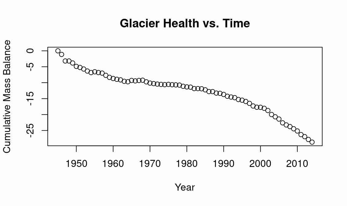
The research does show that glaciers around the world are melting and getting smaller; see, e.g., climate.gov. Tomorrow, we will explore the relationship between shape and glacier health.
2. Working with GIS Data in R
Now that we have some basic data analysis in R under our belt, we start working with GIS data, which is a bit more complex!
Some GIS Data to Play With: Montana Counties
For this tutorial, we will work with GIS data coming from Montana County boundaries. We will download the data directly into R as before, which comes from Montana.gov.
Unfortunately, it is less easy to do so with GIS data than with a standard CSV. First, we download the .zip file into MontanaCounties.zip, and then unzip it in our cloud project:
download.file("https://ftpgeoinfo.msl.mt.gov/Data/Spatial/MSDI/AdministrativeBoundaries/MontanaCounties_shp.zip", destfile = "/cloud/project/MontanaCounties.zip")
system("unzip /cloud/project/MontanaCounties.zip")
You should see the .zip file be downloaded in your working directory, and then the directory MontanaCounties_shp should be created after it is unzipped.
To manipulate shape data, we will use the rgdal and the spatial polygons library. Download and import the library gdal library, and import sp which is a built-in library in R:
NOTE: The rgdal library has recently been retired. Former versions can be downloaded at the address below. We are working actively on a transition to an alternate package.
Old versions of the library are available here. Depending on your setup, it should be possible to install the package using install.packages("rgdal", type="source"). See this forum for troubleshooting until we have a permanent fix.
install.packages("rgdal")
library(rgdal)
library(sp)
Now open the shapefile using the rgdal function readOGR:
counties <- readOGR(dsn="/cloud/project/MontanaCounties_shp/County.shp")
# understand the format of our data
class(counties)
dim(counties)
Expected Output
> class(counties)
[1] "SpatialPolygonsDataFrame"
attr(,"package")
[1] "sp"
> dim(counties)
[1] 56 15                                      NA's   :1
We can see that we’re working now with a new type of data: sp data or “spatial data”. Thankfully, this data inherits lots of the same funtionality from dataframes. We can see that we’re working with a more complex matrix as well; this one has 56 rows and 15 columns.
Unlike our CSV data, shapefile data is much more unweildy. For a better sense of this, take a look at the first few entries of counties:
head(counties, 3)
Clearly, this GIS data is more involved to wrap one’s mind around. However, don’t despair, many others have come before you and successfully dealt with GIS data in R. In fact, R has a built-in function to plot GIS data which is quite satisfying:
plot(counties)
Expected Output
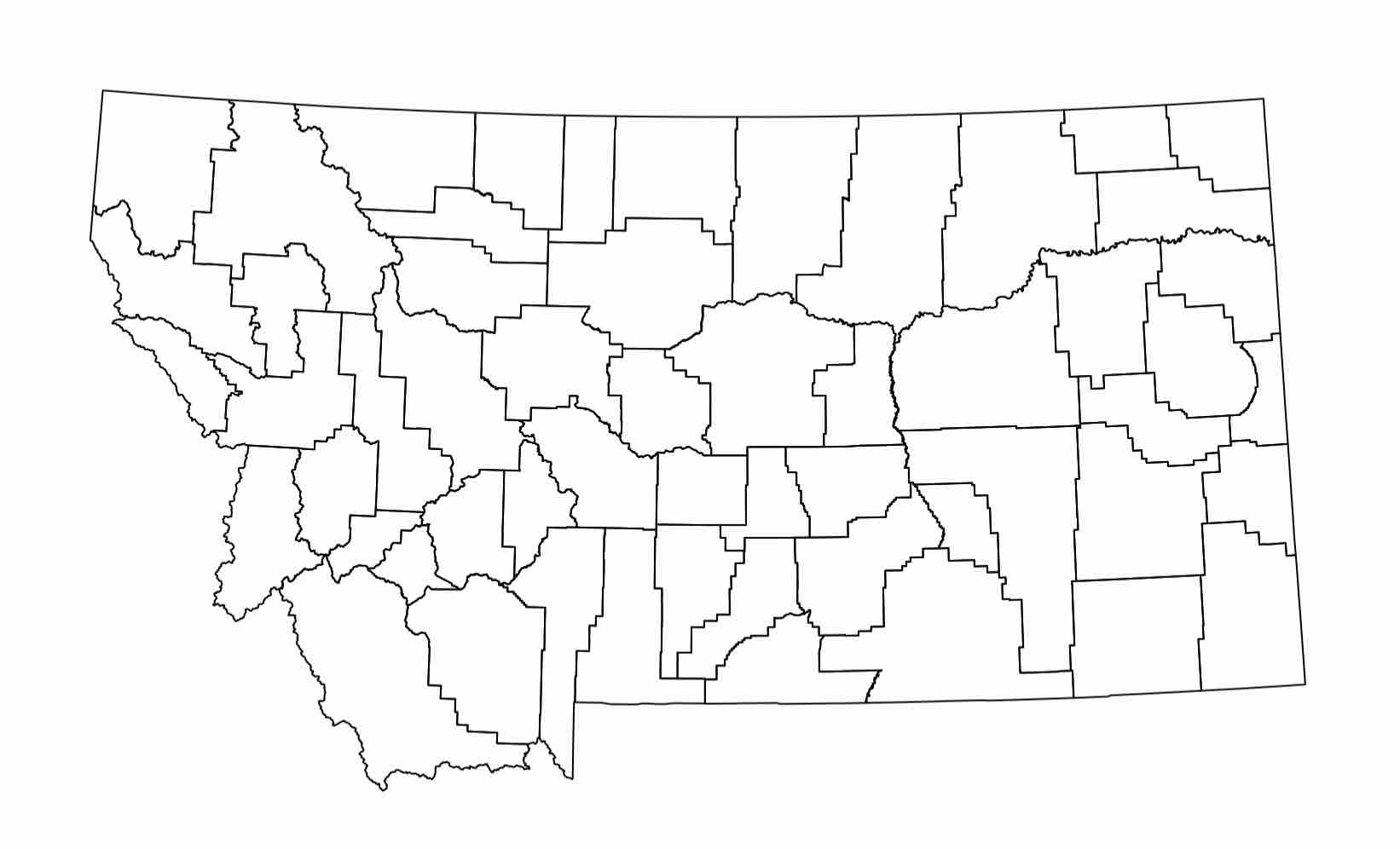
Let’s get a better feel for the data. Intuitively, with this shapefile data there should be, well, a shape … defining each county.
We can get the attributes of spatial polygons data (and most labelled data in R) as follows:
names(counties)
Expected Output
> names(counties)
 [1] "NAME"       "NAMEABBR"   "COUNTYNUMB" "PKEY"       "SQMILES"    "PERIMETER"
 [7] "ACRES"      "ALLFIPS"    "FIPS"       "LAST_UPDAT" "NAMELABEL"  "BAS_ID"
[13] "ID_UK"      "Shape_Leng" "Shape_Area"                                      NA's   :1
Knowing this, we can get the name of every County using the following syntax:
counties$NAME
Expected Output
> counties$NAME
 [1] "CARBON"          "POWDER RIVER"    "MADISON"         "BEAVERHEAD"
 [5] "BIG HORN"        "STILLWATER"      "PARK"            "GALLATIN"
 [9] "SWEET GRASS"     "SILVER BOW"      "CARTER"          "DEER LODGE"
[13] "TREASURE"        "YELLOWSTONE"     "JEFFERSON"       "GOLDEN VALLEY"
[17] "WHEATLAND"       "RAVALLI"         "MUSSELSHELL"     "FALLON"
[21] "BROADWATER"      "ROSEBUD"         "GRANITE"         "CUSTER"
[25] "MEAGHER"         "PRAIRIE"         "JUDITH BASIN"    "WIBAUX"
[29] "PETROLEUM"       "MINERAL"         "POWELL"          "MISSOULA"
[33] "CASCADE"         "FERGUS"          "LEWIS AND CLARK" "GARFIELD"
[37] "LAKE"            "MCCONE"          "TETON"           "CHOUTEAU"
[41] "SANDERS"         "PONDERA"         "ROOSEVELT"       "HILL"
[45] "BLAINE"          "LIBERTY"         "PHILLIPS"        "TOOLE"
[49] "VALLEY"          "DANIELS"         "GLACIER"         "FLATHEAD"
[53] "SHERIDAN"        "LINCOLN"         "DAWSON"          "RICHLAND"
We can also look up the associated data given a county’s index. Try this with Carbon county, at index 1.
counties[1,]
In fact, we can do this with any attribute of the counties data. Play around and get a feel for it! Knowing an attribute of data, we can also find its index. For example, we can find the index of Choteau county by:
which(counties$NAME=="CHOUTEAU")
Expected Output
> which(counties$NAME=="CHOUTEAU")
[1] 40
The which function also has attributes max and min. This allows us to find polygons maximizing and minimizing different attributes. For instance, the index of the county in Montana with smallest perimeter is:
counties$NAME[which.min(counties$PERIMETER)]
Expected Output
> counties$NAME[which.min(counties$PERIMETER)]
[1] "WHEATLAND"
Using what you know about indexing in R, dataframes, and spatial polygons, see if you can find the largest county (by acres) in Montana.
See the Answer
> counties$NAME[which.max(counties$ACRES)]
[1] "BEAVERHEAD"
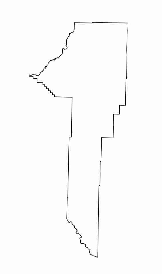
Let’s try to select Gallatin County specifically (which is where you are currently!). Try using the which function to get the associated spatial polygons object.
# save Gallatin County sp object
gallatin <- # HINT: Get the index of Gallatin county, which corresponds to a row in the dataframe
See the Answer
gallatin <- counties[which(counties$NAME=="GALLATIN"),]
And visualize Gallatin County:
plot(gallatin)
Expected Output
More Info
Another popular library for plotting is ggplot2. It has additional parameters you can set to customize the output.install.packages("ggplot2") library(ggplot2) ggplot() + geom_polygon(data = gallatin, aes( x = long, y = lat, group = group), fill="#B9975B", color="#00205B")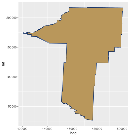
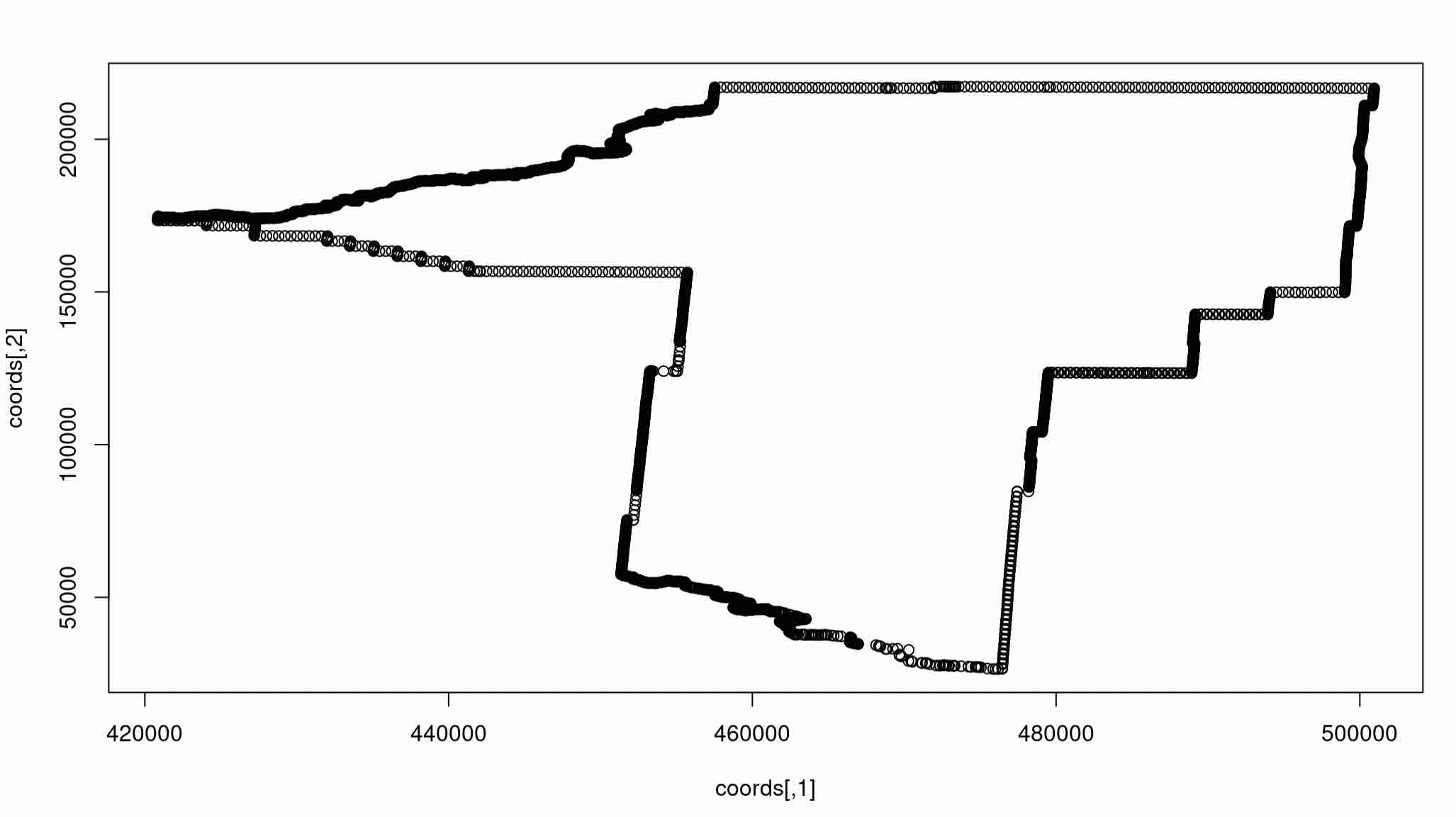
There are tons of things we can do now with an isolated spatial polygon. It should be noted that polygons are defined just as a set of points and a set of edges. We can extract the set of points defining a polygon using some careful syntax:
coords <- gallatin@polygons[[1]]@Polygons[[1]]@coords
plot(coords)
Expected Output
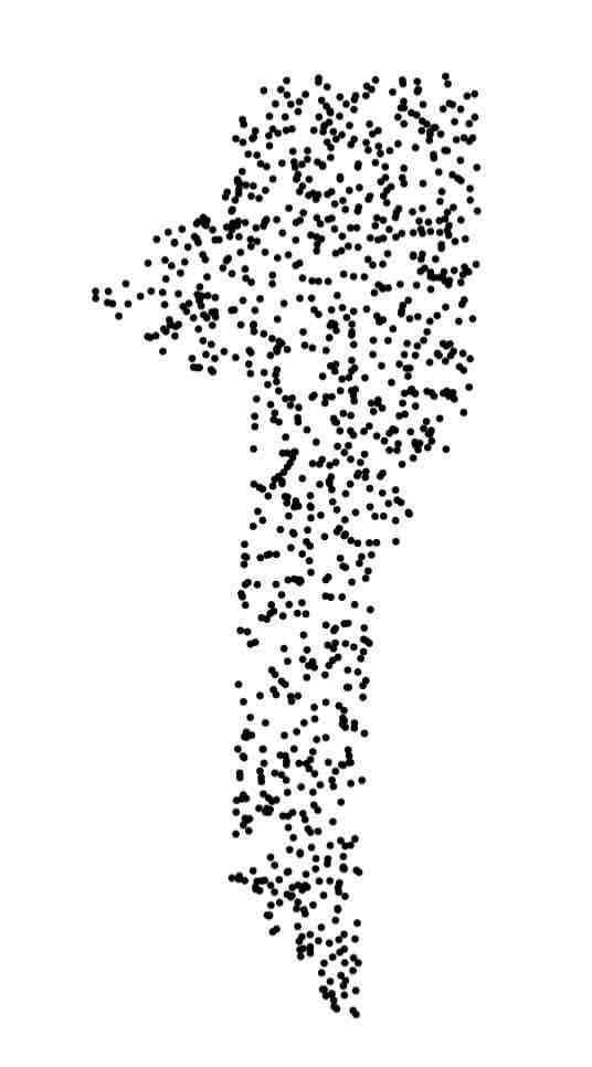
We can also sample within a polygon using the spsample function. Here’s the syntax to do that, and subsequently plot the result:
gallatinSample <- spsample(gallatin,n=1000,"random")
plot(gallatinSample,pch=20,cex=.5)
Expected Output
We can also test whether not a given point lies within Gallatin County using the point.in.polygon function:
point.in.polygon(460000,150000,coords[,1],coords[,2])
point.in.polygon(1,2,coords[,1],coords[,2])
Expected Output
> point.in.polygon(460000,150000,coords[,1],coords[,2])
[1] 1
> point.in.polygon(1,2,coords[,1],coords[,2])
[1] 0
If a point is assigned a 1, then the point lies within the polygon, and if it is a 0, the point lies outside of the polygon. This will be of great importance later on, when we conduct segmentation tasks for topological data analysis. Stay tuned!
Bonus: Multiple Counties
On your own, try selecting the spatial data corresponding to Flathead, Missoula, and Sanders county. (HINT: Remember we can use the which() function to get the index of a given element)
# get the three counties surrounding Lake county, and Flathead lake.
lakeNeighbors <- # select Flathead, Missoula, and Sanders county
See the Answer
lakeNeighbors <- counties[c(which(counties$NAME=="FLATHEAD"), which(counties$NAME=="MISSOULA"), which(counties$NAME=="SANDERS")), ]
If you did this correctly, you should be able to achieve the following plot:
plot(lakeNeighbors)
Expected Output
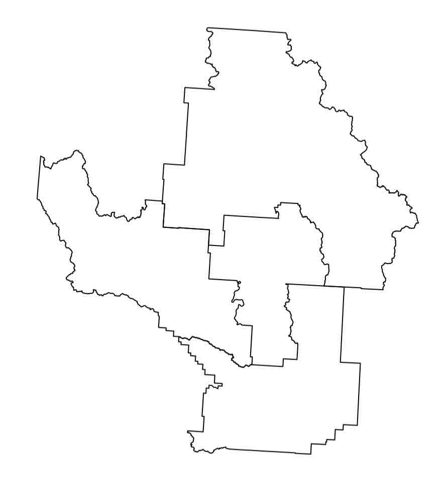
It may look like there are five regions, but the middle one is not a county; it is Flathead Lake!
3. Wrapping Up
Thanks for following along in session 2! To look back on our accomplishments before lunch:
- We learned about basic R programming, data structures, and visualization
- We dealt with GIS data, which is often quite large and contains many fields
- We visualized and played with GIS data
- We extracted the core components in GIS data, the points defining polygons
Enjoy a long lunch in downtown Bozeman! If you have any questions about the above topics, don’t hesitate to ask. And if you have muddy points, post them! Before heading to lunch, remember to save your file.
Credits
- For a more in depth introduction to R, check out the software carpentries tutorials, which are a big inspiration for the style of this workshop
- The glacier CSV data was taken from datahub.io and studies the average mass balance of glaciers worldwide between 1945 and 2014. This data was sourced from the US EPA and the World Glacier Monitoring Service.
- For more on glacier mass balance, see www.antarcticglaciers.org.
- The Montana county shape data was sourced from the Montana state government’s website with data on administrative boundaries
- The heroic mountainscape at the top of the page comes from the National Parks Service, in Glacier National Park.
- The R Graph Gallery has additional tutorials on how to work with shape files in R.