Tutorial on Kernel Density Estimation
Objectives
We want to be able to understand the questions:
- What is a kernel? Not that of your pre popped corn, nor a high ranking military officer, the kind that’s useful when thinking about data.
- How can kernels be of use to understand a set of data?
- What are a few exciting applications of kernel density estimation?
- Every year in Bozeman, Montana, an epic trail race kown as the Bridger Ridge Run takes place in which runners test themselves for 20 grueling miles to see who can most quickly traverse the Bridger Ridge. The citizens of Bozeman, Montana, or “Bozemanites” as they often refer to themselves, carry with them a serious level of pride in their ability to complete these sorts of challenges better than people throughout the rest of the world. As the Bridger Ridge Run has grown into a widely famous race around the country, the superiority of Bozemanites at traversing their beloved ridge is being tested like never before. By the end of this tutorial, we will use Kernel Density Estimation to decide, is there merit to the longheld Bozemanite belief of their ridge traversing superiority, or have the proud people of Bozeman been surpassed by nonlocal runners in this famous ridge traverse?
What is a kernel?
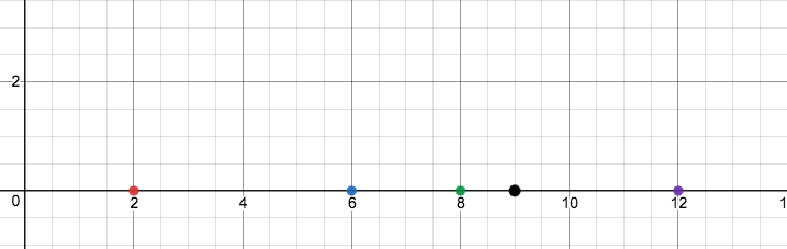
To begin, visualize a number line with points lying along it, as follows:
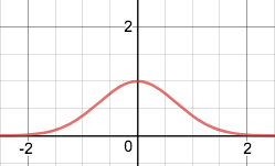
Now, recall a Gaussian curve, the “bell curve” which portrays a normal distribution. The Gaussian curve is visualized by:
With this in mind, visualize the insertion of a Gaussian curve above each point on our data set on the number line:
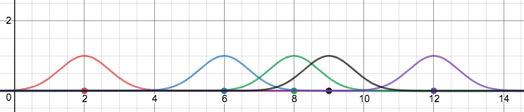
We call the curves inserted above these points kernels. In this example, we’ve chosen to use Gaussian curves as kernels, though other implementations include:
- Rectangular kernels
- Triangular kernels
- Biweight kernels
- Uniform kernels
- Cosine kernels
- Epanechnikov kernels
However, for functional purposes we are primarily concerned with Gaussian and Epanechnikov kernels specifically. We’ve seen some exposure to Gaussian kernels, and Epanechnikov kernels are conceptually quite similar but are parabolic rather than normally distributed in nature.
-
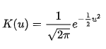
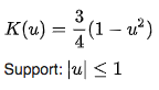
Gaussian kernels are specifically useful since they are naturally distributed. This yields a natural sort of probability in location for each data point, and when taken as a sum of all the points in a data set is actually quite effective in representing the data. A Gaussian kernel K(u) is defined to be:
-
Epanechnikov kernels are useful in their own right, and are representative of data in a manner similar to Gaussian kernels. However, the difference in Epanechnikov kernels lies in their parabolic structure. This is useful for data in which we need to take into account areas with zero density. More formally, this is referred to as compact support, having a closed and bounded domain. When using Gaussian curves, there will always be a nonzero kernel value occupying the space, since Gaussian curves never reach zero. The function for an Epanechnikov kernel K(u) is defined as:
Summing all of our Gaussian kernels together, we gain a nice visualization of the densities of the original points on the number line
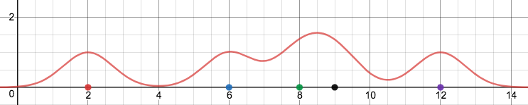
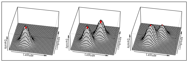
Conceptually, this is the central goal of kernel density estimation. In order to understand sets of data, it is incredibly useful to project their densities in some manner above a set in order to view similarities in their values and to view data in a more probabilistic manner. Adding dimensions, for an n dimensional set of data, we find an n + 1 dimensional kernel density estimate. Thus, for a set of 2 dimensional data, we can construct a similar density visualization in R3.
Consider the position of some occurance of data on a plane. We can visualize the density of that data positionally by different 3 dimensional plots of kernel density, each plot referring to a specific variable which we are concerned with positionally. This graph comes from a paper on geolocation, considering the densities of particular words geographically on Twitter.
Applications of kde
Kernel density estimation is widely applicable as a relatively intuitive, nonparametric method to model the structure of a data set. Below are just a few of countless applications kde can have when interpreting data.
AI
- Image Classification: Unsurprisingly, kernel density estimation is incredibly useful when trying to categorize images. “Nonparametric Kernel Density Estimators for Image Classification” gives a good overview of kernel density estimators for image classification as well as proposing new, nonparametric methods to do so which improve upon existing methods.
- Geolocation: Kernel density estimation is immediately applicable to any sort of map, as it is an easy way to understand the densities of a particular phenomenon in a space. One pertinent example comes with the graph included above, when considering the densities of word use on Twitter in specific regions.
This instance brought up in “Kernel Density Estimation for Text-Based Geolocation” is easily extended to countless data distributed geographically.
Econometrics
- Understanding the probability involved with economic data. Econometricians can utilize kde in order to understand the overall trends in economic data, in hopes to explain the root causes of economic trends. For more information, see
“kde in econometrics”.
—
kde in the R package ‘TDA’
Kernel density estimation can be accomplished by use of the R package ‘TDA’ through the kde function. By this means, it is possible to input data and recieve an actual numerical assessment of kernel density on that data.
The kde function considers:
- Two input matrices, one corresponding to each point in a data set of concern, and the other corresponding to a base grid from which the matrix refers to.
- A smoothing parameter in order to mitigate some level of statistical noise in the data if necessary.
- The type of kernel desired- allowed to be either Gaussian or Epanechnikov
- A weight parameter which allows certain data points to be weighted more or less in the kernel density, prioritizing or deprioritizing aspects of the data if useful
And then returns a vector containing the value of the kernel density estimator at each point in the base grid. This provides a rough quantification of kernel density at each point in a considered space, which is very useful in order to actually use the values associated with a kernel density estimate.

Generic example using points along the unit circle:
library(TDA)
#Generate Data from the unit circle

n <- 300
X <- TDA::circleUnif(n)

#Construct a grid of points over which we evaluate the function

by <- 0.065
Xseq <- seq(-1.6, 1.6, by=by)
Yseq <- seq(-1.7, 1.7, by=by)
Grid <- expand.grid(Xseq,Yseq)

#kernel density estimator

h <- 0.3

KDE <- TDA::kde(X, Grid, h)
Kernel Density Estimation to settle the superiority of Bozemanites in the Bridger Ridge Run:
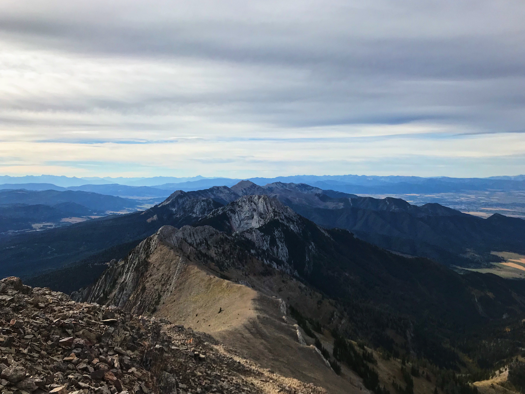
The Bridger Ridge, as seen from just below the summit of Naya Nuki.
To settle once and for all the Bozemanite supremacy in traversing mountain ridges, we can take a look at a kernel density estimation using the times in the 2018 Ridge Run in seconds. The kernel density is constructed with the following code in the R package ‘TDA’.
Sample Code:
#Times of Bozeman runners in top 30 of Ridge Run (in seconds)
RTBOZE <- matrix(c(12909, 13204, 13268, 14497, 14964, 15304, 15350, 15437, 15751, 15752, 15804, 15842, 16754, 16780, 16877, 16978))
by <- 1
xseq <- seq(12900, 17000, by)
Grid <- expand.grid(xseq)
h <- 1

KDEBOZE <- kde(RTBOZE, Grid, h)
#Kernel Density Estimator of Bozeman Runners
#Times of runners in top 30 of Ridge Run from outside of Bozeman (in seconds)
RTOTHER <- matrix(c(14096, 14391, 14678, 14792, 14811, 14940, 15343, 15777, 15797, 15811, 15968, 16605, 16660, 16761))
KDEOTHER <- kde(RTOTHER, Grid, h) ```
Outcome:
While not by any means a complete picture, by considering the kernel density estimation of Bozeman runners vs. runners from outside of Bozeman in the top 30 places in the 2018 Bridger Ridge Run, we can see a slight disparity between the outcomes, which of course, favors Bozemanites.
//TODO: Display findings of estimation graphically, ask Dave // GGPLOT
Works cited:
Hulden, Mans, et al. “Kernel Density Estimation for Text-Based Geolocation.” AAAI Publications, Twenty-Ninth AAAI Conference on Artificial Intelligence, AAAI Conference on Artificial Intelligence, 9 Feb. 2015, www.aaai.org/ocs/index.php/AAAI/AAAI15/paper/view/10034.
Rhodes, Anthony, et al. “Fast On-Line Kernel Density Estimation for Active Object Localization.” ArXiv.org, Cornell University, 16 Nov. 2016, arxiv.org/abs/1611.05369.
Zanin, Adriano, and Ronaldo Dias. “A Review of Kernel Density Estimation with Applications to Econometrics.” ArXiv.org, Cornell University, 12 Dec. 2012, arxiv.org/abs/1212.2812.
All images created with Desmos online calculator